The code/math behind calculating the electron wavefunctions for hydrogen.
Background
I never thought I would have so much fun programming in C++ again. I can’t believe how much I miss operator overloading and templates.
Being able to write ex c = a + b; where a and b are custom types is so nice.
The goal of my next project is creating an interactive display for the electron wavefunctions of hydrogen.
I decided to do this project using GiNaC, and the visualizations will be in three.js (webGL).
Code
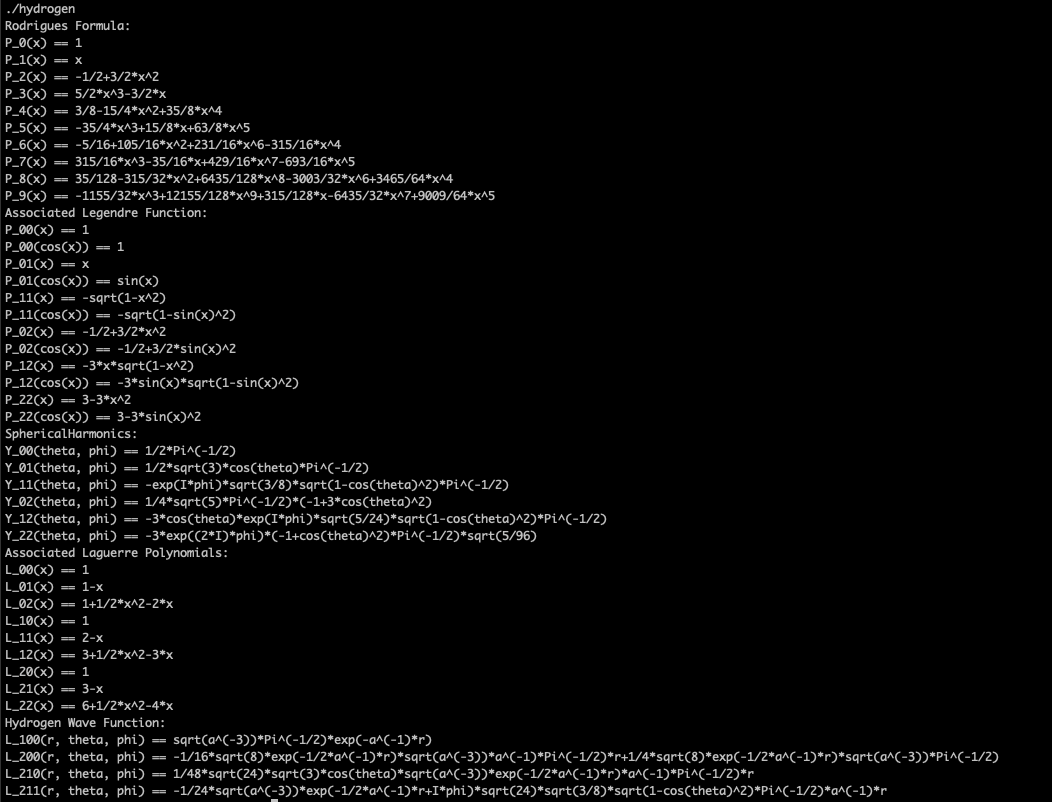
So far I think I have most of the math done:
I’m not 100% sure on the correctness of the final step (HydrogrenWaveFunction), I probably won’t know till I plot them.
But, holy crap GiNaC is cool. I love that I can symbolically create expressions. It makes verifying them much easier. And I can take the derivative of expressions!
Math
Schrödinger Equation in Spherical Coordinates
To find the wavefunctions of hydrogen, you start at the same place you always start at… the Schrödinger Equation!
$$ i \hbar \frac{\partial \Psi}{\partial t} = - \frac{\hbar^2}{2m} \Delta^{2} \Psi + V \Psi $$
For all the examples I’ve been learning about so far, we’ve been using X,Y,Z as the coordinate system. But for hydrogen (and other realistic systems), it makes sense to move to a spherical coordinate system. This is because most real world potentials are proportional to a radius around some origin.
Unfortunately the equation (time-independent Schrödinger Equation in spherical coordinates) gets a bit more complex:
$$ - \frac{\hbar^2}{2m} [ \frac{1}{r^2} \frac{ \partial }{\partial r} ( r^2 \frac{\partial \psi}{\partial r}) + \frac{1}{r^2 \sin{\theta}} \frac{\partial}{\partial \theta} ( \sin{\theta} \frac{\partial \psi}{\partial \theta}) + \frac{1}{r^2 \sin^2{\theta}} ( \frac{\partial^2 \psi}{\partial \phi^2}) ] + V \psi = E \psi $$
Hydrogen Solution
In Hydrogen there’s one proton and one electron. The proton is significantly more massive than the electron. We just pin the proton at the middle and assume the electron floats around. Using Coulomb’s law, we can state that the potential energy of our system will be:
$$ V(r) = -4 \frac{e^2}{4 \pi \epsilon_0 } \frac{1}{r} $$
If you do all the math (and by ‘do the math’, I mean nod along in your text book while crying softly to yourself since you don’t really understand what’s going on), you’ll eventually find that the solutions for a bound electron to hydrogen to be:
$$ \psi*{nlm}(r, \theta, \phi) = \sqrt{ \left(\frac{2}{na}\right)^3 \frac{(n-l-1)!}{2n (n+l)!}} e^{-r/na} \left( \frac{2r}{na}\right)^{l} \left[L*{n-l-1}^{2l+1}(2r/na)\right] Y_l^m(\theta, \phi) $$
Where:
- \( L_{q}^{p} \) is the Associated Laguerre Polynomial, defined by:
$$ L_q^p(x) = \frac{x^{-p} e^x}{q!}\left(\frac{d}{dx}\right)^d (e^{-x}x^{p+q}) $$
-
\( a \) is the Bohr Radius.
-
\( Y_l^m(\theta, \phi) \) is the spherical harmonics, defined by:
$$ Y_l^m(\theta, \phi) = \sqrt{ \frac{(2l+1)}{4 \pi} \frac{(l-m)!}{(l+m)!}} e^{i m \phi} * P^m_l(\cos{\theta}) $$
- \( P^m_l(x) \) is the associated Legendre Polynomials, defined by:
$$ P^m_l(x) = (-1)^m (1-x^2)^{m/2} \left( \frac{d}{dx} \right)^m P_l(x) $$
- \( P_l(x) \) is the Legendre Polynomial, generated by the Rodrigues Formula:
$$ P_l(x) = \frac{1}{2^l l!} \left(\frac{d}{dx}\right)^l (x^2 - 1)^l $$
| n | l | m | $$ \psi_{nlm}(r, \theta, \phi) $$ |
|---|---|---|---|
| 1 | 0 | 0 | $$ \frac{ \exp(-\frac{r}{a}) \sqrt{\frac{1}{a^{3}}}}{\sqrt{\pi}} $$ |
| 2 | 0 | 0 | $$ \frac{1}{4} \frac{ \sqrt{8} \sqrt{\frac{1}{a^{3}}} \exp(-\frac{1}{2} \frac{r}{a})}{\sqrt{\pi}}-\frac{1}{16} \frac{ \sqrt{8} \sqrt{\frac{1}{a^{3}}} \exp(-\frac{1}{2} \frac{r}{a}) r}{ \sqrt{\pi} a} $$ |
| 2 | 1 | 0 | $$ \frac{1}{48} \frac{ \cos(\theta) \sqrt{24} \sqrt{3} r \exp(-\frac{1}{2} \frac{r}{a}) \sqrt{\frac{1}{a^{3}}}}{ \sqrt{\pi} a} $$ |
| 2 | 1 | 1 | $$ -\frac{1}{24} \frac{ \sqrt{24} \sqrt{\frac{3}{8}} \exp(i \phi-\frac{1}{2} \frac{r}{a}) r \sqrt{1-\cos(\theta)^{2}} \sqrt{\frac{1}{a^{3}}}}{ \sqrt{\pi} a} $$ |
| 3 | 0 | 0 | $$ -\frac{10}{729} \frac{ \exp(-\frac{1}{3} \frac{r}{a}) \sqrt{243} r \sqrt{\frac{1}{a^{3}}}}{ \sqrt{\pi} a}+\frac{10}{243} \frac{ \exp(-\frac{1}{3} \frac{r}{a}) \sqrt{243} \sqrt{\frac{1}{a^{3}}}}{\sqrt{\pi}}+\frac{2}{2187} \frac{ \exp(-\frac{1}{3} \frac{r}{a}) \sqrt{243} r^{2} \sqrt{\frac{1}{a^{3}}}}{ \sqrt{\pi} a^{2}} $$ |
| 3 | 1 | 0 | $$ \frac{2}{729} \frac{ \cos(\theta) \sqrt{3} \sqrt{\frac{1}{a^{3}}} r \sqrt{486} \exp(-\frac{1}{3} \frac{r}{a})}{ \sqrt{\pi} a}-\frac{1}{2187} \frac{ \cos(\theta) \sqrt{3} \sqrt{\frac{1}{a^{3}}} r^{2} \sqrt{486} \exp(-\frac{1}{3} \frac{r}{a})}{ \sqrt{\pi} a^{2}} $$ |
| 3 | 1 | 1 | $$ -\frac{4}{729} \frac{ \sqrt{\frac{1}{a^{3}}} \sqrt{\frac{3}{8}} \exp(i \phi-\frac{1}{3} \frac{r}{a}) r \sqrt{1-\cos(\theta)^{2}} \sqrt{486}}{ a \sqrt{\pi}}+\frac{2}{2187} \frac{ \sqrt{\frac{1}{a^{3}}} \sqrt{\frac{3}{8}} \exp(i \phi-\frac{1}{3} \frac{r}{a}) r^{2} \sqrt{1-\cos(\theta)^{2}} \sqrt{486}}{ a^{2} \sqrt{\pi}} $$ |
| 3 | 2 | 0 | $$ -\frac{1}{21870} \frac{ \sqrt{2430} \exp(-\frac{1}{3} \frac{r}{a}) r^{2} \sqrt{5} \sqrt{\frac{1}{a^{3}}}}{ \sqrt{\pi} a^{2}}+\frac{1}{7290} \frac{ \cos(\theta)^{2} \sqrt{2430} \exp(-\frac{1}{3} \frac{r}{a}) r^{2} \sqrt{5} \sqrt{\frac{1}{a^{3}}}}{ \sqrt{\pi} a^{2}} $$ |
| 3 | 2 | 1 | $$ -\frac{2}{3645} \frac{ \cos(\theta) \sqrt{2430} \sqrt{\frac{1}{a^{3}}} \exp(-\frac{1}{3} \frac{r}{a}+i \phi) r^{2} \sqrt{\frac{5}{24}} \sqrt{1-\cos(\theta)^{2}}}{ \sqrt{\pi} a^{2}} $$ |
| 3 | 2 | 2 | $$ -\frac{2}{3645} \frac{ \cos(\theta)^{2} \sqrt{2430} \exp(-\frac{1}{3} \frac{r}{a}+{(2 i)} \phi) r^{2} \sqrt{\frac{5}{96}} \sqrt{\frac{1}{a^{3}}}}{ \sqrt{\pi} a^{2}}+\frac{2}{3645} \frac{ \sqrt{2430} \exp(-\frac{1}{3} \frac{r}{a}+{(2 i)} \phi) r^{2} \sqrt{\frac{5}{96}} \sqrt{\frac{1}{a^{3}}}}{ \sqrt{\pi} a^{2}} $$ |
Building Functions by Differentiation
What’s super cool about a number of those functions is that they’re built using an arbitrary differentiation. \( \left(\frac{d}{dx}\right)^l \).
This is the real reason I chose to use GiNaCs, so I could perform these derivatives symbolically.
GiNaC::ex RodriguesFormula(const GiNaC::symbol &x, int l)
{
    GiNaC::ex diffed = GiNaC::pow(GiNaC::pow(x, 2) - 1, l);
    return GiNaC::normal(1 / (GiNaC::pow(2, l) * GiNaC::factorial(l)) * GiNaC::diff(diffed, x, l));
}
Legendre Polynomials
The Legendre polynomials (and everything built up from it) are cool because they are orthogonal.
This means they can be used to form a basis, and when combining these functions together, they don’t interfere with each other.
This is particularly useful when constructing fourier series, since you can use a set of orthogonal vectors to describe any function. (Commonly Cos / Sin are used, which are also orthogonal. If you look at a chart of Cos/Sin from -pi to pi, and multiply them together and add up the areas, you can convince yourself they equal zero).
What are n, l, and m?
The easiest one to describe is “n”, the principal quantum number. This is the energy state of the wave function. Any wave function with a similar n has the same energy.
The higher the n, the further away the electron is from the nucleus (the proton).
The energy is given by the Bohr formula (which is impressively simple given the wavefunctions we were looking at)
$$ E_n = \frac{E_1}{n^2} $$
\( E_1 = -13.6 eV\), which means that it requires -13.6eV to push an electron completely away from a proton.
l is the Azimuthal Quantum Number, and m is the Magnetic Quantum Number, they both related to the angular momentum of the electron. I might talk more about them in a future blog post.
Up Next
Now that all the math is in code up next is to start plotting the results of these functions. I’m not sure how exactly I want to tackle it, but I think I’ll just random sample a number of points, decide to keep them based off their probability, wait till I get a few hundred each and then just plot those points in three.js.