This post covers a script I wrote for generating the clebsch-gordan coefficients by scratch.

Motivation

We know from classical mechanics that it’s pretty easy to find the composite angular momentum of a system. You just add up all the angular momentum vectors.

Does the same strategy work at the scale of quantum mechanics?

Turns out… not exactly. When adding two particles with different angular momentum, you get a combination of different possible spin/angular momentum results.

Calculating the probabilities of different angular momentums isn’t difficult, but a little tedious, so most people use a special table, commonly referred to as the Clebsch-Gordan coefficients.

As an example, if you had two spin-1 particles and put them in a box and you know the first one has $ m_l = 1 $ and the second has $ m_l == -1 $, we can look up and see that:

$$ \Ket{1\ 1\ 1\ -1} = \sqrt{\frac{1}{6}}\Ket{2\ 0} + \sqrt{\frac{1}{2}} \Ket{1\ 0} + \sqrt{\frac{1}{3}}\Ket{0\ 0}$$

Where the first ket is the two particles $ \Ket{l_1\ l_2\ m_1\ m_2} $, and the following kets are the composite angular momentums $ \Ket{l\ m} $.

The goal of this post is to generate that table.

Background

Basis

Using Bra-ket notation, we usually represent the angular momentum and spin of a system like:

$$ \ket{l\ m_l} \quad \Ket{s\ m_s} $$

$ l $ and $ s $ can somewhat be thought of as the total angular momentum/spin possible of the system, and $ m_l $ and $ m_s $ is the value in a specific direction (usually picked to be z).

As an example, an electron is a spin 1/2 particle that we usually call spin up or spin down. So a spin up electron can be represented as:

$$ \ket{e_{up}} = \Ket{\frac{1}{2}\ \frac{1}{2}} $$

Operators

There’s a couple of questions we can ask of our system. Ideally we’d like to know the angular momentum vector, but sadly that’s not possible as seen by the commutation relation for angular momentum $ [L_x, L_y] = i \hbar L_z $, where $ L_x $ is the operator that tells us the angular momentum in the z direction $ L_z \Ket{l\ m_l}_z = \hbar m \Ket{l\ m_l}_z $.

(It’s also a very curious fact that both angular momentum and spin are described by the same algebra. $ [S_x, S_y] = i \hbar S_z $.)

But getting back on track, we can only know one component of the angular momentum vector. But thankfully there is something else that commutes with the individual operators… $ L^2 $. (In group theory this is called the Casmir operator, more info in a previous blog post). The eigenvalue of the $ L^2 $ operator gives us a scalar with the total angular momentum of the particle.

So in total we can know the angular momentum in one direction (z) and the total angular momentum. These are the $ l $ and $ m_l $ values from earlier.

There’s two other operators that will be essential later, the ladder operators for angular momentun. $ L_{+}, L_{-} $. These ladder operators are similar to the ladder operators from the harmonic oscillator. Using them we can go up and down in angular momentum values ( $ m_l $).

$$ L_{-} \Ket{l\ m} = \hbar \sqrt{s(s+1) - m(m-1)} \Ket{l\ m-1} $$

Plan of attack

Just a reminder, the goal is to find the total angular momentum of a system composed of two particles. Each pair of angular momentums is its own table.

Very similar to how we found the energy levels of the quantum harmonic oscillator, we’re going to start with the highest possible energy level and then repeatedly apply the lowering operator $ L_{-} $ until we fall off.

Given two particles, the highest possible composite angular momentum is the direct sum. $ m = m_1+m_2 $ and $ l_{max} = l_1 + l_2 $.

So we start there.

$$ \Ket{l_1\ l_2\ m_1\ m_2} = \Ket{l_{max}\ m} $$

Tools we’ll need

A matrix library that can build tensor product states

We need to build tensor states with the two particles. Thankfully I already built a library to do this for my quantum computing simulations.

We also need something that can decompose the tensor states into a human readable form.

Generate $ L $ matrixes for different representations

We need a way to generate the $ L $ matrixes in different representations, i.e. different matrix sizes for the different sizes of $ l_1 $ and $ l_2 $. You can see them for a few of the representations here.

This isn’t too hard if we’re smart about it.

We already know $ L_z $ since we work in the z-basis. So the diagonal elements are the eigenvalues of $ m_l $.

The ladder operators are also easy, we know what the eigenvalues are $ L_{-} \Ket{l\ m} = \hbar \sqrt{s(s+1) - m(m-1)} \Ket{l\ m-1} $, so we just put those in the correct spots in the matrix (upper right corner such that m -> m+1 or bottom left corner such that m -> m-1).

Then we are pretty much done, since $ L_{+} = L_x + i L_y $ and $ L_{-} = L_x - i L_y $ we can get $ L_x = \frac{1}{2} (L_{+} + L_{-}) $ and $ L_x = \frac{1}{2} (L_{+} + L_{-}) $.

Gram-Schmidt

But there’s a slight wrinkle in our ladder plan. Applying the ladder operator will only give us one of the vectors in the lower subspace (the highest spin state). So at each level we actually need to find the other orthogonal states. Thankfully Gram-Schmidt comes to the rescue.

There’s one other minor wrinkle with using Gram-Schmidt. Our basis states are in the full tensor space of the two particles, but we need to make sure that we Gram-Schmidt in only the subspace. We can kind of cheat in code and “highlight” the specific entries we are interested in, and the rest of the states will be ignored by the algorithm.

// Gram-Schmidt
export function find_orthogonal_vector_in_subspace(vectors: Matrix[]): Matrix {
  let out = Matrix.zero(1, vectors[0].height());
  // Highlight the related orthogonal states
  for (let a of vectors) {
    for (let i = 0; i < a.height(); i++) {
      if (!a.at(0, i).equals(new Complex(0, 0))) {
        out.set(0, i, new Complex(1, 0));
      }
    }
  }

  // Perform Gram-Schmidt
  for (let a of vectors) {
    let proj = a.mulScalar(out.adjoint().mulMatrix(a).at(0, 0));
    out = out.sub(proj).normalize();
  }
  return out;
}

Results

It works! Here’s the results for 3/2 x 1:

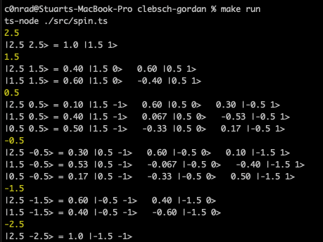
The code is a little sloppy, but can be found here: https://github.com/c0nrad/sims/blob/master/clebsch-gordan/src/spin.ts

What went well

I learned a lot, and I’m much more comfortable with quantum angular momentum
My quantum computing libraries worked out of the box for tensor products and matrix multiplications
It’s super cool that you can use some basic group theory to construct the $ L $ operators.

What did’t go well

It took awhile to really grok the Clebsch-Gordan table, I should have spent a little bit more time up front understanding what I really was trying to do. I didn’t understand it as well as I thought

Future

I’m guessing I’ll eventually need this for some particle simulations in the future. So this library will sit on the shelf until then.

Up next I think will be some stat mech simulations.

c0nrad's c0rner

Learning and learning

Sim 4: Clebsch-Gordan Coefficients