We derive wien’s constant using plank’s blackbody radiation formula.
Overview
I had to memorize Wien’s constant for the physics GRE. At the time I had a lot to memorize so I didn’t think much of it, but it was a little strange that Wien’s constant wasn’t given in terms of some other variables. For example, fine structure constant is roughly 1/137, but it comes from \( \frac{e^2}{4 \pi \epsilon_0} \frac{1}{\hbar c} \).
But after digging deeper, it turns out that Wien’s constant can’t be given in terms of other constants! But we can still derive it (numerically).
In this post we will (1) talk about Plank’s Distribution Law (2) talk about Wien’s law (3) do a couple of quick examples (4) derive Wien’s constant (5) try out sympy and see if it makes deriving Wien’s constant any easier
Plank’s Law
Oddly enough, one of the big problems that spurred in the quantum revolution of the early 1900s was the calculation of black body radiation. All objects are constantly radiating some form of electromagnetic radiation, where the intensity and wavelength of radiation depends on temperature.
The current model at the time was known as “Rayleigh-Jeans law”. It worked well at low frequencies, but quickly diverged at high frequencies giving rise to infinite intensities. This was known as the ultraviolet catastrophe.
Plank proposed something radical; he quantized the energy. Instead of treating energy as continuous, he discretized it, and lo and behold the divergence went away.
$$ u(\lambda, T) = \frac{8 c^{2} h \pi}{\lambda^{5} \left(e^{\frac{c h}{T k \lambda}} - 1\right)} $$
Plank’s law for a few temperatures can be seen here ( source):
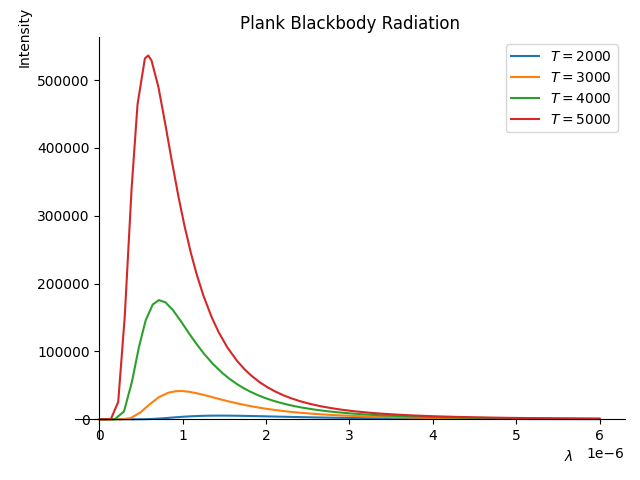
As an example, a campfire burns at roughly 1200K. Most of the radiation is coming out as infra-red (the right side of the chart). It’s not the visibile (left side of chart) component that keeps you warm.
Wien’s Law
Wien’s law gives you the peak wavelength of black-body radiation for different temperatures. It’s a very simple equation:
$$ \lambda_{peak} = \frac{2.9 * 10^{-3}}{T} $$
As a simple example, the sun roughly burns at 5800K, which equates to a peak wavelength of 500 nm (blue), which is (not) coincidentally in the visible spectrum. It was very nice of the sun to output mostly in the spectrum that our eyes can see! (just kidding Darwin).
Calculating Wien’s constant
Where did the constant \( 2.9 * 10^{-3} \) in Wien’s law come from? Why don’t we represent it using fundamental constants?
Well, it turns out it’s not possible, at least not in a way similar to the fine structure constant. There’s a step in the derivation where we have to numerically solve an equation.
Let’s calculate the Wien constant. As a reminder, we want the “peak” (highest intensity) for each wavelength/temperature pair. We can find the maximum (peak) by finding where the derivative is zero.
$$ \frac{\partial}{\partial \lambda} \frac{8 c^{2} h \pi}{\lambda^{5} \left(e^{\frac{c h}{T k \lambda}} - 1\right)} = 0$$
So after taking the derivative of the Plank Blackbody Equation we get:
$$ \frac{40 c^{2} h \pi}{\lambda^{6} \left(e^{\frac{c h}{T k \lambda}} - 1\right)} + \frac{8 c^{3} h^{2} \pi e^{\frac{c h}{T k \lambda}}}{T k \lambda^{7} \left(e^{\frac{c h}{T k \lambda}} - 1\right)^{2}} $$
After substituting \( u = \frac{c h}{T k \lambda} \) and solving for u we get:
$$ u = W\left(- \frac{5}{e^{5}}\right) + 5 \approx 4.965 $$
Where W is the Lambert W function. This is why we can’t write out a closed form solution, the equation is transcendental. W is the inverse of \( u e^u \).
But now we’re done!
$$ u = \frac{c h}{T k \lambda} \approx 4.965 $$ $$ \lambda = \frac{0.0029}{T} $$
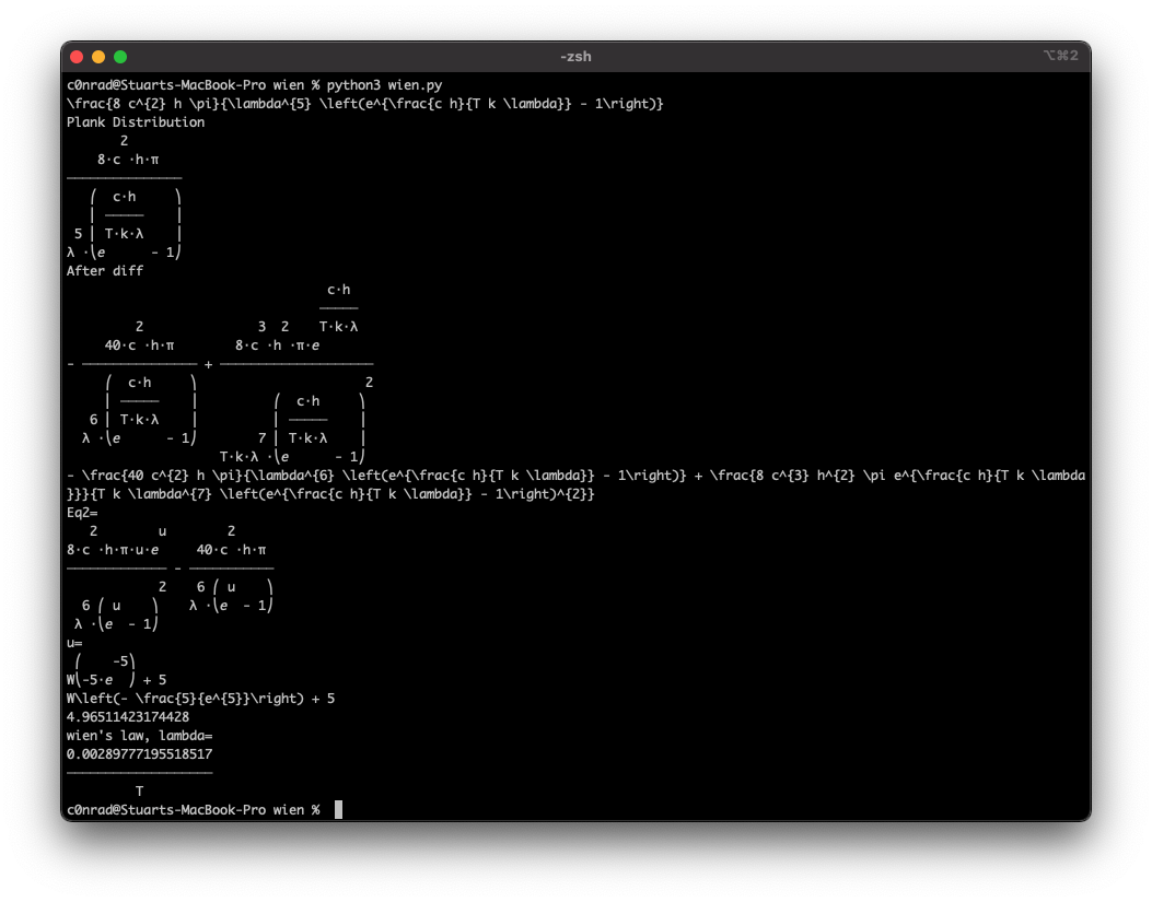
Solution using Sympy
It was my first time using sympy. I have mixed feelings about it. I had to tinker a lot with the substitutions to get it to solve what I wanted, and I was worried it wouldn’t be able to solve it at all. (At first it was just hanging and I had no idea if it would ever complete). I spent a good hour just tinkering with it, whereas I wouldn’t be surprised if mathematica just solved it directly.
But, having the computation natively in python is such a huge plus. I’ll probably reach to sympy when I know the equations aren’t too hard or I need to connect to external systems/resources. But mathematica will probably be my go to when the equations get tough.
Conclusion
Overall, it was a fun project. I wish I could have been there during the beginnings of the quantum revolution. But I guess you never really know you’re in the revolution until it’s over.
I’m not sure what project I’ll tackle next. I’ve been looking at some lattice gauge calculations, and PBS Spacetime just published a neat video on DFT which might be fun to try.