Day one of building 99 simulations. We’ll reduce a problem that at first requires 6 parameters with coupling, to a problem with just 3 (or 2, depending on how you look at it) by exploiting the symmetry. “Nature does not care how we describe her”.
Why 99 simulations
I’ve been doing the previous qualification exams on Yale’s website as practice for graduate school. And to be honest, I’m so bored. I really don’t enjoy sludging through problems. I think I’m a decent programmer, and I got that way because I truly do enjoy doing programming problems. And because I enjoy the programming challenges, I do them. But with physics problems I’m always dragging my feet. I think in a perfect world I’d have infinite motivation to sit down for 10 hours a day and do problems, but I’m not perfect.
So to compromise, instead I’m going to try to take all the topics on Yale’s qualifying exam, and try to simulate them, and also write a little blog post about some of the math. Hopefully this way I’ll at least enjoy learning some new physics topics. Eventually I’ll need to go back and actually practice solving problems, but I’ll pass that hurdle later. Until then, I’d just like to have fun learning in my free time.
For the first topic, I’m taking a look at two body central force problems.
Two Body Central Force Problems
A number of important systems are two body central force systems. Examples include modeling hydrogen’s electron and proton ( previous sim), modeling planetary bodies (earth-moon or sun-earth), and more.
Modeling these problems just using their position and velocity can get a little tricky. Writing a simple \( r_1(t) \) requires knowledge of \( r_2(t) \) which is also coupled to \( r_1(t) \). The solution will not be simple. But instead if we abuse some symmetry and choice of coordinates, we can model the system in a much simpler way.
Central Force
Two common central forces are gravity and electric charge (Coulomb). These forces are “conservative” (1. force only depends on \( \vec{r} \) 2. the work between any two points is the same along any path. Friction is not a conservative force since not all paths are the same).
If we look at the potential for both gravity and coulomb’s law we’ll notice something peculiar about the r terms.
$$ U_{gravity}(r_1, r_2) = \frac{G m_1 m_2}{ |r_1 - r_2|} $$
$$ U_{coulomb}(r_1, r_2) = \frac{1}{4 \pi \epsilon_0} \frac{q_1 q_2}{ |r_1 - r_2|} $$
Both the equations only depend on the relative distance between the objects. So instead of modeling the potentials as \( U(\vec{r_1}, \vec{r_2}) \) we could instead model the potential with the relative position \( \vec{r} = |\vec{r_1} - \vec{r_2}| \), so \( U(\vec{r}) \).
So now our Lagrangian has two parameters:
$$ L = \frac{1}{2} m_1 \dot{r}^2_1 + \frac{1}{2} m_2 \dot{r}^2_2 - U(\vec{r}) $$
But we can do better!
Reference Frame, Center of Mass
We get to choose our frame of reference. So, we could be naive and imagine the two bodies moving through space and rotating around each other, or we could make it easy and define our coordinate system such that the two bodies are spinning around a constant point.
This constant point is the center of mass \( \vec{R} = \frac{m_1 \vec{r_1} + m_2 \vec{r_2}}{m_1 + m_2} \).
We can now rewrite \( \vec{r_1} \) and \( \vec{r_2} \) in terms of \( \vec{R} \) and \( \vec{r} \).
$$ \vec{r_1} = \vec{R} + \frac{m_2}{M} \vec{r} \qquad \vec{r_2} = \vec{R} - \frac{m_1}{M}\vec{r} $$
So now if we substitute this into our Lagrangian:
$$ L = \frac{1}{2} m_1 \dot{r}^2_1 + \frac{1}{2} m_2 \dot{r}^2_2 - U(r) $$ $$ L = \frac{1}{2} m_1 (\dot{R} + \frac{m_2}{M}\dot{r})^2 + \frac{1}{2} m_2 (\dot{R} - \frac{m_1}{M}\dot{r})^2 - U(r) $$ $$ L = \frac{1}{2} (M \dot{R}^2 + \mu \dot{r}^2) - U(r) $$
Where we define \( \mu \) as the reduced mass \( \mu = \frac{m_1 m_2}{m_1 + m_2} \).
We can also just set our center of mass to be zero in the coordinate system, and then the lagrangian is even simpler!
Solving the Lagrangian
We have two coordinates, \(R\) and \(r\). Plugging the first coordinate into the euler-lagrange equation we get:
$$ \frac{d}{dt} \frac{\partial L}{\partial \dot{R}} = \frac{ \partial L}{\partial R} $$
$$ \frac{d}{dt} M \dot{R} = 0 $$
Momentum is conserved.
Plugging in the second coordinate:
$$ \frac{d}{dt} \frac{\partial L}{\partial \dot{r}} = \frac{ \partial L}{\partial r} $$
$$ \frac{d}{dt} \mu \dot{r} = -\frac{\partial U(r)}{\partial r} $$
Newton’s equation with reduced mass instead of mass for a single particle!!
We can reduce it even further, but I’ll save that for the next project. For now let’s build a simulation of what we have so far.
Simulation
https://blog.c0nrad.io/sims/twobody/
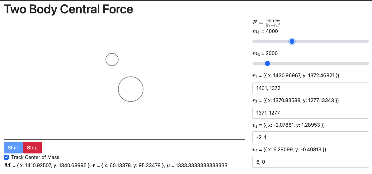
This simulation tracks the movements of two bodies under the influence of a central force. Under the hood the simulation uses semi-implicit euler. It calculates the center of mass, reduced mass, and relative position vector.
On the technical side it’s using paperjs for the canvas and angular for the UI.
What went well
- paperjs was pretty simple to use. I’m only drawing circles, but it did what I needed it to do
- Tracking center of mass is pretty cool. I’m slightly cheating by just moving the viewport, but it wouldn’t be hard to actually change the frame of reference
- It’s a good base simulation for moving on to more exciting simulations! (tracking the potential and different conic sections)
Random Thought
Converting the problem to center of mass and relative position really reminds me of doing the change of basis to normal modes when doing coupled oscilators. Maybe I’ll go back later and see if this can be represented as an eigenvalue problem and deduce the CM and relative position coordinates.
Conclusion
A fun first project. I’m excited to build further on the simulation with conic sections and potential graphs.